A Practical Guide to Robot Programming in Python

Simulation gives developers a safe, practical entry point into robot programming without putting any physical hardware at risk. It allows control logic to be tested repeatedly and for experiments to be reset quickly when the robot behaves unexpectedly.

Python remains one of the most widely used programming languages in robotics. In this tutorial, we’ll use Python and Webots to explore reactive control, a fundamental part of mobile robotics, despite advances in AI and autonomous navigation. You can think of reactive control as learning how to steer a car before learning GPS navigation.

We’ll program a differential-drive robot that uses proximity sensors to detect obstacles and wheel encoders to estimate its position. The completed controller will guide the robot toward a destination and adjust its movement when the route is blocked. The approach I’ve taken here draws on my experience studying robotics at Carnegie Mellon University’s Robotics Institute and, later, working on behavior prediction for self-driving cars at Waymo, where I saw the same principles applied in modern autonomous systems.

You don’t need an advanced background in mathematics or robotics to follow this tutorial. Basic knowledge of Python, trigonometry, vectors, and simple mathematical calculations is sufficient. Familiarity with object-oriented programming is helpful, but not essential.

What Are Robots Used For Today?

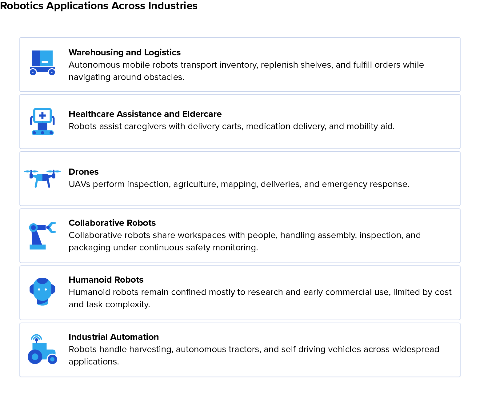
Robots are increasingly used where automation can improve consistency or reduce human exposure to hazardous environments. Today, robotics supports work across industries including healthcare, logistics, agriculture, and manufacturing. Some robots perform repetitive tasks in highly controlled environments, while others must respond to changing conditions.

Here’s an overview of the most common applications.

The Fundamental Challenge of Robot Programming

A central challenge in robotics is that a robot can’t directly observe the true state of the world; it relies on sensor data, which is often imperfect.

Robots operate in physical environments. Consider a robot approaching a wall: It doesn’t know the wall’s exact distance or angle, or even its own precise position. It may also be unaware that the floor is slippery or that another object has moved since the previous control cycle. The robot therefore responds to its best estimate of the world, based on observations that may be incomplete or delayed.

It’s a common misconception that sensors provide exact measurements. Every sensor has limitations, including restricted resolution and field of view, and sensitivity to environmental conditions. Small measurement errors can accumulate quickly, and a robot may gradually estimate itself several centimeters from its true position.

I find that developers coming from conventional software engineering are often surprised that the hardest problems are not always programming errors. The code may execute exactly as intended, yet the robot can still behave incorrectly because its sensors are noisy or its model of the world is imperfect. Effective robot production, therefore, requires developers to account for uncertainty as carefully as they write the code itself.

Choosing a Robot Simulator

If you want to learn and test robot control logic safely, simulation is usually the fastest way to iterate on control algorithms. Making mistakes in a simulation environment avoids damaging expensive hardware, reducing equipment and repair costs. Experiments can also be reset and repeated quickly, and debugging is considerably easier.

Recommended Robot Simulators

The right simulator will depend heavily on your project. Below I outline several widely used options and the types of robotics work they support:

• Webots: Webots is widely regarded as one of the most approachable robotics simulators for novices, but it’s capable enough for many research and educational applications. It’s a great choice for rapid prototyping and lightweight projects, as it is relatively easy to install, and it provides an integrated development environment with excellent documentation. It supports Python, offers built-in robot models, a Robot Operating System 2 (ROS 2) interface, and is open source.
• Gazebo: Often the default simulator for ROS 2 tutorials, it integrates naturally with tools such as ros2_control, Nav2, SLAM Toolbox, and RViz. For ROS 2 development, this is a strong choice.
• Isaac Sim: Developed by NVIDIA, it targets high-fidelity robotics simulation and AI-driven robotics workflows. For reinforcement learning, synthetic data generation, photorealistic rendering, and industrial and humanoid robotics, this is a good fit. It has become a leading platform for researchers working on learning-based robotics because it supports large-scale data generation and accelerated simulation.

For this tutorial, we’ll use Webots, as its Python support and built-in e-puck model provide a practical environment for learning reactive control.

Setting Up the Robotic Programming Project in Webots

Before getting started, make sure you have Webots installed and configured. If you haven’t installed it yet, follow the Webots installation instructions first.

Next, we’ll create a small project and separate the robot interface, behaviors, and state estimation into reusable modules. Separating sensor access, robot behaviors, and state estimation mirrors the way larger robotics systems are structured.

1. First, create a project folder in your integrated development environment (IDE), for example, robot_tutorial.
2. Then create a new Webots project using that folder, and create a new world by selecting File > New > New World File.
3. Add an e-puck robot to the scene by selecting Add > Robots > e-puck. Copy the Python files from this tutorial into the generated controller directory, and assign the robot_tutorial controller to the robot.

An empty world containing only the e-puck is sufficient for the first tests. Obstacles can be added later when implementing obstacle avoidance.

Your project in your IDE should look like this:

my_project/
├── controllers/
│   └── robot_tutorial/
│       ├── robot_tutorial.py
│       ├── robot.py
│       ├── odometry.py
│       ├── behaviors.py
│       ├── robot_controller.py
│       └── constants.py
└── worlds/
    └── my_world.wbt

Throughout this tutorial, we’ll gradually construct a simple reactive controller for a differential-drive robot. Rather than writing the entire program at once, each implementation section develops one part of the controller:

• robot.py communicates with the simulator and exposes the robot’s sensors and motors.
• odometry.py estimates the robot’s pose from wheel encoder readings.
• behaviors.py implements the Go-to-Goal, Avoid-Obstacles, and Follow-Wall behaviors.
• robot_controller.py selects which behavior should be active using a finite state machine.
• robot_tutorial.py ties everything together inside the robot’s control loop.

Start with constants.py, which contains the controller settings and robot parameters used throughout the project:

## Shared constants for the reactive navigation controller and robot parameters used by the controller.

# Webots control period (ms)
TIME_STEP = 64

# e-puck geometry (meters)
WHEEL_RADIUS = 0.0205
AXLE_LENGTH = 0.052

# Motion limits
MAX_LINEAR_SPEED = 0.12 # m/s
MAX_ANGULAR_SPEED = 4.0 # rad/s

# e-puck wheel motor limit (rad/s)
MAX_WHEEL_SPEED = 6.28

# Controller gains
GO_TO_GOAL_GAIN = 2.5
WALL_FOLLOW_GAIN = 6.0

# Goal position
GOAL_X = 1.0
GOAL_Y = 1.0

# Goal considered reached within this radius (meters)
GOAL_TOLERANCE = 0.05

# IR thresholds
OBSTACLE_THRESHOLD = 80
TARGET_WALL_READING = 70

For the results shown here, the robot starts at the world’s origin facing the positive x-axis. If you move or rotate the robot before starting the simulation, its trajectory will be different.

Our Example Robot and Its Sensors

This tutorial uses a simple differential-drive mobile robot equipped with infrared proximity sensors and wheel encoders. These sensors illustrate the core principles of perception, control, and state estimation.

A differential-drive mobile robot is one of the most common robot designs in both education and industry. It typically has two independently driven wheels, one or more passive caster wheels or a skid for balance, and no steering mechanism. It changes direction by varying the speed of its left and right wheels.

Proximity Sensors and Wheel Encoders

Robots such as the one we are simulating in this tutorial rely on two sensor types: infrared proximity sensors and wheel encoders. Each serves a different purpose:

• Infrared proximity sensors let the robot detect nearby obstacles. These sensors don’t identify what the obstacle is, however, they simply provide an estimate of how close an object is within their operating range.
• Wheel encoders measure how much each wheel has rotated. The robot uses this information to estimate the distance traveled, its change in heading, and its approximate position. Unlike proximity sensors, encoders track the robot’s motion instead of its surroundings.

Sensor Modernization and Sensor Fusion

This tutorial uses infrared proximity sensors because they are simple and inexpensive. More advanced mobile robots often supplement them with light detection and ranging (LiDAR), depth cameras, and inertial measurement units (IMUs).

Relying on a single sensor type can make a robot vulnerable in real environments. Infrared sensors have a short range and can be affected by surface properties or ambient light. LiDAR measures distances more accurately, but it can’t identify object types and may be affected by weather.

Sensor fusion is the process of merging data from several sensors to create a more accurate and trustworthy estimate of the robot’s state or surroundings than could be obtained from any one sensor alone. For example, LiDAR can provide accurate distance measurements while an IMU tracks changes in motion and orientation. Combining their data allows each sensor to compensate for limitations in the other.

Implementing the Robot Interface

The only component that depends on Webots is the robot interface. Its purpose is to hide the simulator-specific API from the navigation algorithms. The rest of the controller will communicate with the robot exclusively through this interface.

In robot.py, add the code below. The temporary print() statements display the motor objects and calculated wheel speeds in the terminal, which can help identify setup errors.

## Webots robot interface.

from dataclasses import dataclass

from controller import Robot
from constants import (
    TIME_STEP,
    WHEEL_RADIUS,
    AXLE_LENGTH,
    MAX_WHEEL_SPEED,
)


@dataclass
class SensorData:
    ## Current robot sensor measurements.
    ir: list[float]
    left_encoder: float
    right_encoder: float


class RobotInterface:
    def __init__(self):
        self.robot = Robot()

        # Motors
        self.left_motor = self.robot.getDevice("left wheel motor")
        print(self.left_motor)
        self.right_motor = self.robot.getDevice("right wheel motor")
        print(self.right_motor)

        self.left_motor.setPosition(float("inf"))
        self.right_motor.setPosition(float("inf"))
        self.left_motor.setVelocity(0.0)
        self.right_motor.setVelocity(0.0)

        # Wheel encoders
        self.left_encoder = self.robot.getDevice("left wheel sensor")
        self.right_encoder = self.robot.getDevice("right wheel sensor")
        self.left_encoder.enable(TIME_STEP)
        self.right_encoder.enable(TIME_STEP)

        # Infrared proximity sensors
        self.ir_sensors = []
        for i in range(8):
            sensor = self.robot.getDevice(f"ps{i}")
            sensor.enable(TIME_STEP)
            self.ir_sensors.append(sensor)

    def step(self):
        ## Advance the simulation one timestep.
        return self.robot.step(TIME_STEP) != -1

    def read(self):
        ## Read all robot sensors.
        ir = [sensor.getValue() for sensor in self.ir_sensors]
        return SensorData(
            ir=ir,
            left_encoder=self.left_encoder.getValue(),
            right_encoder=self.right_encoder.getValue(),
        )

    def drive(self, linear_velocity, angular_velocity):
        print("Driving", linear_velocity, angular_velocity)

        left_speed = (
            linear_velocity
            - angular_velocity * AXLE_LENGTH / 2
        ) / WHEEL_RADIUS
        right_speed = (
            linear_velocity
            + angular_velocity * AXLE_LENGTH / 2
        ) / WHEEL_RADIUS

        left_speed = max(
            -MAX_WHEEL_SPEED,
            min(MAX_WHEEL_SPEED, left_speed),
        )
        right_speed = max(
            -MAX_WHEEL_SPEED,
            min(MAX_WHEEL_SPEED, right_speed),
        )

        print("Wheel speeds:", left_speed, right_speed)
        self.left_motor.setVelocity(left_speed)
        self.right_motor.setVelocity(right_speed)

    def stop(self):
        self.left_motor.setVelocity(0.0)
        self.right_motor.setVelocity(0.0)

The Control Loop

The control loop is a continuous cycle in which the robot uses sensor measurements to decide how to move, observes the result, and adjusts its next action.

If you’ve written game software before, this structure will probably feel somewhat familiar. Just like a game loop, the robot repeatedly reads inputs, updates its internal state, and produces outputs. The main difference is that every output changes the physical world, which becomes the input to the next iteration.

This is what happens at every stage of the cycle:

• Sense: The robot collects information from its sensors. This can include infrared proximity sensors, wheel encoders, but also GPS (outdoors), LiDAR scans, camera images, and IMU measurements. This is the data gathering stage.
• Think: The controller processes the collected data and runs the control algorithm. It may determine whether an obstacle is nearby, calculate the direction of the goal, or assess whether the robot is moving as expected.
• Act: The controller sends commands to the motors. In this example, those commands determine the speed of the left and right wheels. The resulting movement changes what the robot observes during the next control cycle.
• Sense again: The robot repeats the cycle, sensing changes since the last control cycle and adjusting its behavior accordingly.

Unlike most traditional software programs that execute a task and then terminate, a robot controller must keep repeating its feedback loop for as long as the robot operates.

The loop must also execute at a consistent rate. In this project, the controller updates every 64 milliseconds, or approximately 15.6 times per second. This continuous feedback allows the robot to recover from errors.

Imagine the robot wants to drive toward a goal. Initially, the controller may command both wheels to move forward. Moments later, one wheel turns slightly more slowly than the other because of a variation in the motors’ response. Even if the difference is very small, the robot is now drifting off course.

At the next control cycle, the wheel encoders will record the difference in rotation. The controller will update the robot’s estimated heading, identify the error, and adjust the steering commands. In other words, the robot continuously corrects itself.

Understanding Movement With the Unicycle Model

Thinking about movement is complicated. Even if the robot has two independently driven wheels, controlling those wheels directly is not always the easiest way to understand movement.

Robotics often uses the unicycle model, which describes motion using two intuitive quantities:

• Translational (linear) velocity, usually written as v
• Angular velocity, usually written as ω

The controller can then describe movement in terms of how fast the robot should move forward and how quickly it should rotate.

Translational velocity (v) describes forward or backward motion in meters per second. If (v = 0), the robot doesn’t move forward or backward. It moves forward when (v > 0) and backward when (v < 0).

Angular velocity (ω) describes the speed at which the robot turns, measured in radians per second. If (ω = 0), the robot drives straight ahead. A positive value rotates the robot left, while a negative value rotates it right.

Estimating the Robot’s State

Up to this point, the tutorial has shown how a robot gathers sensor data and uses a control loop to decide how to move. The controller also needs an estimate of where the robot is. A robot doesn’t know its exact location. It continuously builds and updates an internal estimate from sensor data, a process known as state estimation. We can divide state estimation into two related tasks: estimating the environment and self-localization.

When estimating the environment, the robot uses its proximity sensors to estimate what is around it and choose the appropriate behavior. Importantly, the robot doesn’t build a detailed map at this stage. It simply reacts to what it currently detects.

The robot also needs to estimate its own movement. This estimate is based on wheel encoder measurements, a process known as odometry.

Odometry and Pose Estimation

Odometry measures the movement of a robot’s wheels over time to estimate its position. The robot doesn’t measure its position directly; it calculates how far it has traveled since the previous control cycle and updates its estimated location accordingly.

Odometry is a type of dead reckoning in which the current position is calculated based on a known starting point and measured motion.

The robot’s pose describes both its position and orientation. For a robot moving on a flat floor, the pose is usually represented as x, y, θ, where:

• x is the horizontal position.
• y is the vertical position.
• θ is the heading angle.

The Webots position sensors used in this tutorial measure each wheel’s angular position in radians.

From Wheel Rotation to Distance

During each update, the controller subtracts the previous sensor reading from the current reading to calculate the wheel’s change in angle, Δφ (here, Δ refers to a change and φ refers to the wheel’s rotation angle). The controller then converts this angular movement into linear distance using the wheel radius:

d = r × Δφ

where d is the distance traveled by the wheel and r is the wheel radius.

For the e-puck wheel radius of 0.0205 meters, a rotation of one radian corresponds to 0.0205 meters, or 2.05 centimeters, of travel.

Differential-drive Odometry

Because the robot has two wheels that are independently driven, it compares their motions.

Let:

• dL = distance traveled by the left wheel
• dR = distance traveled by the right wheel

The average forward motion is:

d = dL + dR 2

where d is the forward distance traveled by the robot’s center.

If both wheels move exactly the same distance, the robot moves straight ahead. If one wheel moves farther than the other, the robot must also have rotated.

The change in heading is estimated as:

Δθ = dR − dL L

where L is the distance between the wheels and Δθ is the change in the robot’s orientation.

This equation is one of the fundamental relationships in differential-drive kinematics.

Odometry Drifts and Probabilistic Robotics

Odometry becomes less accurate over time because every pose estimate depends on measurements that contain small errors. Each new estimate is calculated from the previous one, so those errors accumulate as the robot moves. This gradual accumulation of errors is called odometry drift. Once an error enters the position estimate, each and every subsequent calculation begins from an incorrect position.

Errors can be caused by:

• Wheel slip
• Uneven surfaces
• Mechanical imperfections
• Sensor noise
• Numerical approximation

Because these errors are unavoidable, modern robotics systems model the uncertainty associated with each estimate, which is known as probabilistic robotics. The robot maintains both an estimate of its current state and a measure of how confident it is in that estimate. As odometry drift increases, uncertainty about the robot’s position grows. Additional sensor data can then help narrow the range of possible positions.

Two approaches to probabilistic state estimation are:

• Kalman filters combine what the robot expects to happen based on its motion model (such as odometry) with what its sensors are actually measuring. If one source of information is less reliable, the filter gives it less weight when estimating the robot’s state.
• Particle filters use a collection of separate hypotheses, or particles, to represent the robot’s possible locations. As new sensor measurements arrive, likely particles are reinforced and unlikely particles are discarded. This makes particle filters particularly useful when the robot could plausibly be in several locations.

Implementing Odometry and Pose Estimation

The next step is to estimate the robot’s pose. We’ll implement this logic in a dedicated odometry.py module so the rest of the controller doesn’t need to know how the estimate is calculated.

from dataclasses import dataclass
from math import cos, sin, pi

from constants import (
    WHEEL_RADIUS,
    AXLE_LENGTH,
)


@dataclass
class Pose:
    x: float = 0.0
    y: float = 0.0
    theta: float = 0.0


class Odometry:
    def __init__(self):
        self.pose = Pose()
        self.previous_left = None
        self.previous_right = None

    @staticmethod
    def normalize(angle):
        while angle > pi:
            angle -= 2 * pi
        while angle < -pi:
            angle += 2 * pi
        return angle

    def update(self, left_encoder, right_encoder):
        if self.previous_left is None:
            self.previous_left = left_encoder
            self.previous_right = right_encoder
            return self.pose

        delta_left = left_encoder - self.previous_left
        delta_right = right_encoder - self.previous_right

        self.previous_left = left_encoder
        self.previous_right = right_encoder

        d_left = delta_left * WHEEL_RADIUS
        d_right = delta_right * WHEEL_RADIUS

        distance = (d_left + d_right) / 2.0
        rotation = (d_right - d_left) / AXLE_LENGTH

        midpoint_theta = self.pose.theta + rotation / 2.0

        x = self.pose.x + distance * cos(midpoint_theta)
        y = self.pose.y + distance * sin(midpoint_theta)
        theta = self.normalize(self.pose.theta + rotation)

        self.pose = Pose(x, y, theta)
        return self.pose

Core Robot Behaviors

A robot’s behavior is a self-contained control strategy designed to achieve a specific objective. For example, an Avoid-Obstacles behavior aims to prevent collisions. Each behavior receives information about the robot’s current state and produces a desired movement command.

The behaviors don’t directly control the motors. They generate high-level motion commands, expressed as linear and angular velocities, which are later converted into wheel speeds.

Go-to-Goal Behavior

The robot’s default navigation strategy is Go-to-Goal behavior, which steers it toward the target whenever the path ahead is clear and continues until it reaches its destination.

The controller determines the goal direction by first comparing the robot’s current position (xr, yr) with the goal position (xg, yg).

The vector pointing toward the goal is:

Δx = xg − xr

Δx = yg − yr

The desired heading is then computed using the two-argument arctangent function:

θgoal = atan2(Δy, Δx)

The simplest way to steer the robot is using a proportional (P) controller. The controller compares the direction toward the goal with the robot’s current heading. The difference between these two directions is called the heading error, eθ.

eθ = normalize(θgoal − θ)

The angular velocity of the command is:

ω = Kpeθ

where Kp is the proportional gain, and eθ is the heading error. The smaller the heading error, the gentler the steering, and vice versa. This creates smooth turning rather than abrupt direction changes.

A useful trick is to reduce forward speed when the robot needs to make a sharp turn. If the heading is almost correct, the robot can continue at close to its maximum speed. As the heading error increases, the following calculation reduces its linear velocity:

v = vmax / (1 + 2|e|)

This prevents the robot from continuing at full speed while facing away from the goal.

Avoid-Obstacles Behavior

The Avoid-Obstacles behavior generates a steering command that guides the robot away from nearby objects before a collision occurs. It responds immediately to the latest sensor data without planning a complete path around the obstacle.

The controller compares weighted readings from sensors on the robot’s left and right sides. If the sensors on the right detect a stronger obstacle signal, the robot turns left. If the readings are stronger on the left, it turns right. This uses the same general principle as potential-field navigation, although the simplified controller doesn’t calculate complete repulsive vectors.

The controller assigns a different weight to each sensor. For example, the front sensor might have a high weight, while a side sensor might have a low one. Sensors that detect obstacles directly ahead typically have the most influence because they represent the highest collision risk. The safest steering direction is determined by combining the weighted measurements.

Follow-Wall Behavior

Obstacle avoidance works well for isolated objects, but it can struggle with larger obstacles such as a long wall blocking the route. If the robot only alternates between Go-to-Goal and Avoid-Obstacles, it may repeatedly steer toward the goal, encounter the wall, turn away, then immediately steer back toward the wall.

This is where the Follow-Wall behavior comes in. It allows the robot to move around a large obstacle while maintaining a roughly consistent distance from it, which prevents continuous oscillation.

A simple proportional controller can again be used, this time to maintain a target infrared sensor reading:

ω = Kpe

where:

• ω is the angular velocity (how quickly the robot turns).
• Kp is the proportional gain that determines how strongly the robot reacts to the error.
• e is the difference between the desired distance from the wall and the measured distance.

This lets the robot follow the wall by adjusting its steering in response to the sensor measurements.

Of course, the robot can’t follow the wall forever. In this simplified controller, it periodically checks whether it is approximately facing the goal again and whether the path ahead is clear. Once both conditions are met, control returns to the Go-to-Goal behavior.

Implementing Behaviors

With the robot’s pose estimate and sensor readings available, we can implement the three navigation behaviors. Each function returns the linear and angular velocities required by the controller. In behaviors.py, add the following code:

from math import atan2, pi

from constants import (
    GOAL_X,
    GOAL_Y,
    GO_TO_GOAL_GAIN,
    OBSTACLE_THRESHOLD,
    MAX_LINEAR_SPEED,
    MAX_ANGULAR_SPEED,
    TARGET_WALL_READING,
    WALL_FOLLOW_GAIN,
)


def normalize_angle(angle):
    while angle > pi:
        angle -= 2 * pi
    while angle < -pi:
        angle += 2 * pi
    return angle


# Go-to-Goal
def go_to_goal(pose):
    dx = GOAL_X - pose.x
    dy = GOAL_Y - pose.y

    desired_heading = atan2(dy, dx)
    heading_error = normalize_angle(
        desired_heading - pose.theta
    )

    angular_velocity = (
        GO_TO_GOAL_GAIN * heading_error
    )
    angular_velocity = max(
        -MAX_ANGULAR_SPEED,
        min(MAX_ANGULAR_SPEED, angular_velocity),
    )

    # Slow down while making large turns.
    linear_velocity = (
        MAX_LINEAR_SPEED
        / (1.0 + 2.0 * abs(heading_error))
    )

    return linear_velocity, angular_velocity


# Avoid-Obstacles
def avoid_obstacles(sensor_data):
    # Steer away from nearby obstacles using weighted
    # infrared sensor readings.
    ir = sensor_data.ir

    # Front-facing sensors receive larger weights because
    # they represent the greatest collision risk.
    left = (
        3 * ir[7]
        + 2 * ir[6]
        + 1 * ir[5]
    )
    right = (
        3 * ir[0]
        + 2 * ir[1]
        + 1 * ir[2]
    )

    obstacle_detected = (
        max(
            ir[0], ir[1], ir[2],
            ir[5], ir[6], ir[7],
        )
        > OBSTACLE_THRESHOLD
    )

    steering = 0.003 * (right - left)

    # Turn right when an obstacle is directly ahead and
    # the left and right readings are nearly balanced.
    # This leaves the obstacle on the robot's left side
    # for the Follow-Wall behavior.
    if obstacle_detected and abs(steering) < 0.1:
        steering = -MAX_ANGULAR_SPEED

    steering = max(
        -MAX_ANGULAR_SPEED,
        min(MAX_ANGULAR_SPEED, steering),
    )

    linear_velocity = 0.05

    return (
        obstacle_detected,
        linear_velocity,
        steering,
    )


# Follow-Wall
def follow_wall(sensor_data):
    ir = sensor_data.ir

    # Use the left-side sensors to follow the boundary.
    wall_reading = (
        ir[6] + ir[7]
    ) / 2.0

    error = TARGET_WALL_READING - wall_reading

    angular_velocity = (
        WALL_FOLLOW_GAIN
        * error
        * 0.01
    )
    angular_velocity = max(
        -MAX_ANGULAR_SPEED,
        min(MAX_ANGULAR_SPEED, angular_velocity),
    )

    linear_velocity = 0.06

    return (
        linear_velocity,
        angular_velocity,
    )

Core Robot Behaviors: Key Takeaways

• Robot behaviors convert pose estimates and sensor readings into linear and angular velocity commands, which the robot interface then translates into wheel speeds.
• Go-to-Goal behavior corrects the robot’s heading toward its destination and reduces its forward speed during sharper turns.
• Avoid-Obstacles behavior gives greater weight to sensors facing the highest collision risk and steers away from stronger readings.
• Follow-Wall behavior maintains a target distance from an obstacle until the robot faces the goal and has a clear route forward.

Combining Behaviors: The Hybrid State Machine

None of these behaviors is sufficient on its own. Successful navigation depends on switching between them at the appropriate time.

A finite state machine (FSM) determines which behavior should be active based on the robot’s current state and sensor data. Because each discrete state activates a continuous control behavior, this architecture can also be described as a hybrid state machine.

A state machine represents the robot as being in one of several discrete states. In this tutorial, those states are:

• Go-to-Goal
• Avoid-Obstacles
• Follow-Wall

Let’s look at a typical navigation task:

• Step 1: The robot begins moving toward the goal (State = Go-to-Goal).
• Step 2: An obstacle is identified directly ahead (State = Avoid-Obstacles). The robot steers away.
• Step 3: The obstacle turns out to be a long wall. Avoiding it again in the same way would cause oscillation (State = Follow-Wall). The robot moves around the large obstacle maintaining a safe distance.
• Step 4: After a while, the robot is again approximately facing the goal and the path ahead is clear (State = Go-to-Goal). It leaves the wall and resumes traveling toward the destination.

Implementing FSM

The FSM assigns each behavior to a state and switches between them when the relevant transition conditions are met. In robot_controller.py, add the following code:

from enum import Enum, auto
from math import atan2, hypot, pi

from constants import (
    GOAL_X,
    GOAL_Y,
    GOAL_TOLERANCE,
    OBSTACLE_THRESHOLD,
)
from behaviors import (
    go_to_goal,
    avoid_obstacles,
    follow_wall,
)


class State(Enum):
    # Navigation states
    GO_TO_GOAL = auto()
    AVOID_OBSTACLE = auto()
    FOLLOW_WALL = auto()


class ReactiveController:
    # Selects the active behavior during each control cycle.
    def __init__(self):
        self.state = State.GO_TO_GOAL

    @staticmethod
    def normalize_angle(angle):
        # Normalize an angle to [-π, π].
        while angle > pi:
            angle -= 2 * pi
        while angle < -pi:
            angle += 2 * pi
        return angle

    def obstacle_detected(self, sensors):
        # Check the sensors covering the robot's left
        # and right sides.
        return (
            max(
                sensors.ir[0],
                sensors.ir[1],
                sensors.ir[2],
                sensors.ir[5],
                sensors.ir[6],
                sensors.ir[7],
            )
            > OBSTACLE_THRESHOLD
        )

    def path_ahead_clear(self, sensors):
        # Check the sensors facing the path ahead.
        return (
            max(
                sensors.ir[0],
                sensors.ir[1],
                sensors.ir[6],
                sensors.ir[7],
            )
            <= OBSTACLE_THRESHOLD
        )

    def goal_reached(self, pose):
        # Return True if the robot has reached the goal.
        distance = hypot(
            GOAL_X - pose.x,
            GOAL_Y - pose.y,
        )
        return distance < GOAL_TOLERANCE

    def aligned_with_goal(self, pose):
        # Return True if the robot is approximately
        # facing the goal.
        desired_heading = atan2(
            GOAL_Y - pose.y,
            GOAL_X - pose.x,
        )
        error = self.normalize_angle(
            desired_heading - pose.theta
        )
        return abs(error) < 0.3

    def compute(self, pose, sensors):
        # Stop once the goal has been reached.
        if self.goal_reached(pose):
            return 0.0, 0.0

        # Go-to-Goal
        if self.state == State.GO_TO_GOAL:
            if self.obstacle_detected(sensors):
                self.state = State.AVOID_OBSTACLE
                _, linear, angular = avoid_obstacles(
                    sensors
                )
                return linear, angular

            return go_to_goal(pose)

        # Avoid-Obstacles
        if self.state == State.AVOID_OBSTACLE:
            detected, linear, angular = avoid_obstacles(
                sensors
            )

            # Continue avoiding the obstacle while it
            # remains near the robot.
            if detected:
                return linear, angular

            # Begin following the obstacle boundary.
            self.state = State.FOLLOW_WALL
            return follow_wall(sensors)

        # Follow-Wall
        if self.state == State.FOLLOW_WALL:
            # Resume direct navigation once the robot
            # faces the goal and the path is clear.
            if (
                self.aligned_with_goal(pose)
                and self.path_ahead_clear(sensors)
            ):
                self.state = State.GO_TO_GOAL
                return go_to_goal(pose)

            return follow_wall(sensors)

        # Fallback
        return 0.0, 0.0

Putting Everything Together

With the robot interface, odometry, navigation behaviors, and FSM complete, the final controller is quite compact. In robot_tutorial.py, add the following code:

from robot import RobotInterface
from odometry import Odometry
from robot_controller import ReactiveController


def main():
    robot = RobotInterface()
    odometry = Odometry()
    controller = ReactiveController()

    while robot.step():
        # Read sensors.
        sensors = robot.read()

        # Estimate pose.
        pose = odometry.update(
            sensors.left_encoder,
            sensors.right_encoder,
        )

        # Compute velocity command.
        linear_velocity, angular_velocity = (
            controller.compute(
                pose,
                sensors,
            )
        )

        # Drive robot.
        robot.drive(
            linear_velocity,
            angular_velocity,
        )

    robot.stop()


if __name__ == "__main__":
    main()

To test the complete controller, add one or more solid obstacles between the robot’s starting position and the goal. Include a long obstacle or wall if you want to observe the transition to Follow-Wall behavior.

If everything has been implemented correctly, the robot should behave approximately as follows:

1. It begins driving toward the goal.
2. When the front infrared sensors detect an obstacle, it switches to obstacle avoidance.
3. Once the obstacle is no longer directly ahead, it begins following the obstacle boundary.
4. When it is approximately facing the goal again and the path ahead is clear, it resumes driving toward the destination.
5. After entering the goal region, the controller commands zero linear and angular velocity, and the robot stops.

Once the controller is assigned to the robot, press Run in Webots. The simulator will execute robot_tutorial.py.

When and Why Robot Controllers Fail

Failure modes are a day-to-day reality, even with well-tuned reactive controllers. Robotics takes place in an uncertain physical environment, and the controller can only respond to the information available to it.

The following failure modes show how limitations in the controller and changes in its environment can prevent the robot from behaving as intended:

• Local minima: One of the classic problems in reactive navigation is becoming trapped in a local minimum. Consider a robot trying to reach a goal behind a U-shaped obstacle. It may reach a position where moving toward the goal leads into the obstacle, but moving away increases its distance from the goal.
• Oscillation: This commonly results from poorly coordinated behaviors, such as a robot repeatedly alternating between Go-to-Goal and Avoid-Obstacles when it encounters a large obstacle.
• Sensor limitations: A controller can only respond to the information it receives. Reflective surfaces may confuse infrared sensors, for example, while a temporary sensor failure can leave the controller with incomplete information.
• Dynamic environments: Moving people, vehicles, or other robots can change the environment faster than the controller can update its estimate or select an appropriate response.
• Accumulated estimation errors: Odometry drift and inaccurate sensor measurements can gradually cause the robot’s estimated pose to diverge from its actual position.
• Parameter sensitivity: Values that work well in one environment may require adjustment in another. Testing and tuning are therefore normal parts of robotics development.

How This Tutorial Relates to ROS 2

ROS 2 is a widely used framework for connecting and managing the software components in a robot. Some beginners may believe they need to learn ROS 2 before they can learn robotics, but that’s not necessarily true. By learning the basic robotics concepts first, you learn how a robot uses sensor data to decide how to move. ROS 2 then gives you a framework for connecting the software components involved.

Mapping the Tutorial Architecture to ROS 2

The architecture developed in this tutorial maps naturally to ROS 2’s distributed programming model:

In this tutorial, everything (sensors, state estimator, supervisor, behavior, motors) runs inside a single Python program. In ROS 2, those responsibilities are usually separated into different nodes, such as an encoder node, localization node, supervisor node, controller node, and motor driver node. The control loop still exists, although it is distributed across those nodes.

When a Lightweight Python Simulator Is the Right Choice

A lightweight simulator is a good choice when learning the fundamental concepts or prototyping a small controller. It avoids the additional configuration involved in a distributed ROS 2 system, allowing the control logic and its effect on the robot to remain visible in one program.

When to Move to ROS 2

Moving to ROS 2 is usually driven by project requirements. It becomes useful when the robot needs multiple software components, computers, or hardware devices to communicate through a shared framework.

Consider moving to ROS 2 for:

• Coordinating multiple robots: ROS 2 provides a standard mechanism for exchanging information between multiple robots and computers.
• Processing multiple data streams: ROS 2 offers a modular architecture that favors this sort of task.
• Using more sophisticated software: ROS 2 was designed to be modular and scalable.
• Integrating hardware: Real robots typically contain many independent hardware devices (motor controllers, cameras, arms, GPS receivers, etc.). ROS 2’s common ecosystem is designed to integrate these devices using standardized interfaces and existing drivers.

What Comes After Reactive Control?

Throughout this tutorial, the robot has relied on reactive control, using current sensor data to select its behavior and respond to nearby obstacles. This provides a foundation for autonomous navigation, but more advanced systems also need to understand their position within a wider environment and plan beyond their immediate sensor readings.

Localization, Path Planning, and SLAM

Once the robot knows where it is, path planning comes into play. A planner uses the available map to select a route to the destination. This gives the robot a wider view of the environment than reactive control, which responds to immediate sensor measurements.

When no map is available, the robot has to solve two problems: building a map and determining where it is within the map. This is known as simultaneous localization and mapping (SLAM).

These two problems have a circular dependency: The robot needs to know where it is to build an accurate map, and it needs the map to determine where it is. SLAM estimates the robot’s pose and the surrounding environment together, often combining inputs from wheel odometry, IMUs, LiDAR, or cameras.

A good example of this is a modern robot vacuum, which needs to create a map of your apartment the first time you take it out of the box. With every new cleaning session, it refines its map.

Reactive control still has a role within this more advanced navigation system. Even with an accurate map and planned route, the robot must respond to people, pets, and other obstacles that move unexpectedly.

Learning-based Approaches in Modern Robot Programming

In addition to classical control and planning algorithms, modern robotics increasingly incorporates machine learning. By using data and experience, engineers can train robots to make decisions without explicitly programming them.

One of the most important approaches is reinforcement learning (RL). In RL, instead of telling the robot exactly what to do and how to move, the developer lets the robot learn through repeated interaction with an environment. By performing an action, observing the outcome, and receiving feedback (a reward or penalty), it gradually improves its behavior. The outcome is like a policy that maps its observations into actions.

Training often takes place in simulation, which creates a sim-to-real gap when the policy is transferred to physical hardware. Techniques such as domain randomization, realistic sensor models, and fine-tuning on physical robots can help the policy adapt to conditions that were absent from the simulation.

Nowadays, machine learning is an important tool in robotics, but it doesn’t replace classical robotics. It’s particularly valuable for perception, where deep learning supports object detection, image segmentation, visual localization, and scene understanding.

Machine learning can also support adaptive control by helping robots respond to changing payloads, wheel wear, or terrain conditions. Some research systems train a single neural network that maps sensor inputs directly to control commands. These are called end-to-end policies, and they require large amounts of data.

Building on the Foundations of Robot Programming

The controller built in this tutorial is deliberately simple, but it demonstrates the continuous feedback loop that connects sensor measurements to motor commands through an evolving estimate of the robot’s state. Its limitations also show why testing and adjustment are fundamental parts of robot programming.

Once you’re comfortable with the controller, you can experiment with its proportional gains or modify the rules that trigger each behavior. Sensor fusion and path planning can extend its navigation capabilities, and ROS 2 provides a framework for coordinating the same responsibilities across a larger system. More advanced robots may use richer sensors or learning-based techniques, but the principles developed here continue to shape how they perceive and respond to the world.